
A grid-tied solar plant is not sized from the roof outwards. It is sized from the point of interconnection inwards, and that single reversal is where most commercial and industrial projects go wrong.
The usual sequence is familiar. A factory owner looks at a 2,800 m² roof, divides by the area of a module, and arrives at a number in the hundreds of kilowatts. A proposal is written against that number, the modules are ordered, and somewhere in the paperwork the utility returns an interconnection approval for half the requested capacity, the existing transformer turns out to be loaded already, and the inverter is now larger than anything the grid will accept. The array is built, the plant is capped at 55% of its nameplate output by the export controller, and nobody can explain why the payback moved from four years to seven.
This guide covers grid-tied solar plants from 50 kW to 1 MW, the band where a factory, a commercial building or a small utility customer owns the roof and the meter but not the grid. It works through the four ceilings that actually determine capacity — interconnection approval, transformer rating, self-consumption shape and inverter ratio — and then walks a 300 kW rooftop example from the first bill to the final layout.
The interconnection limit sets your capacity, not the roof area
The number that governs a grid-tied plant is the capacity the network operator will allow at the connection point, and in most commercial projects it is smaller than the roof and smaller than the load.
Three interconnection modes exist, and each one changes the sizing arithmetic.
| Interconnection mode | What the meter sees | Capacity ceiling | Where it fits |
|---|---|---|---|
| Full export | All generation flows to the grid | Approved export capacity | Ground-mounted plants selling power |
| Self-consumption with export | Import and export both metered | An export limit set by the utility | Commercial sites with strong daytime load |
| Zero export | Import only; output is curtailed above site load | Site load at every 15-minute interval | Weak or saturated networks that reject new generation |
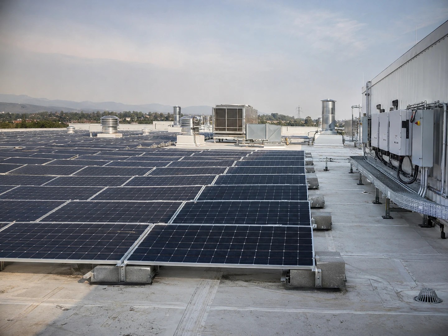
The third mode is increasingly common, and it is the one that catches designers by surprise. A zero-export approval does not cap the array at the site’s average load. It caps instantaneous output at the site’s load in each 15-minute interval, including the lunch break when the factory’s machines stop and the roof is still at full production.
The practical consequence is that two plants with the same 300 kW AC approval can differ by 60% in annual yield depending on whether they may export. A site with an 08:00 to 18:00 load profile and an export ban will spill its production between 11:00 and 14:00 unless storage is added, while the same array at the same site with export allowed will sell the surplus at whatever the feed-in tariff pays.
Our engineering team’s assessment of a factory solar project starts from the utility’s answer, not the roof measurement, because the answer is the one that cannot be negotiated after the steel is up.
Ask for the interconnection approval in writing before the layout is frozen. The document should state three things: the approved AC capacity at the point of connection, whether export is permitted and at what limit, and the protection and metering requirements the utility will enforce. If it states only the first, the project is not yet defined.
A DC/AC ratio above 1.35 costs you clipping revenue
The DC/AC ratio is installed module capacity divided by inverter AC rating, and it exists because a solar array almost never produces its nameplate output.
Modules are rated at standard test conditions — 1,000 W/m² irradiance, 25°C cell temperature. A real roof reaches that irradiance for a short window on clear days and spends the rest of the year below it, and the cells run 20 to 30°C hotter than ambient, which cuts output by roughly 0.35% per degree. An array rated 405 kWp might peak at 330 kW on a cool clear afternoon and spend most of its year below 250 kW.
Sizing the inverter to the array nameplate means the inverter sits at part load for its entire life. Sizing the array above the inverter means the inverter runs at its rated output during the best hours, and only the excess is clipped.
The question is how much clipping is worth accepting.
| DC/AC ratio | Clipping loss, moderate irradiance | Clipping loss, high irradiance | Comment |
|---|---|---|---|
| 1.10 | Below 1% | 1–2% | Inverter rarely at rating; capital-heavy |
| 1.20 | 1–2% | 2–3% | Conservative default for cloudy climates |
| 1.35 | 2–4% | 4–6% | Common for commercial roofs |
| 1.50 | 5–8% | 9–13% | Only where module cost is very low |

The values are indicative and depend on the site’s irradiance distribution, ambient temperature and module temperature coefficient. They are not a substitute for an hourly simulation, but they are close enough to settle the argument.
The economics that justify a high ratio are simple. Modules cost less per watt than inverters, and an inverter running at 95% of its rating for 1,200 hours a year produces more energy than one running at 70% for the same period. A ratio of 1.35 typically delivers 3 to 5% more annual yield per dollar of inverter capacity than a ratio of 1.10, at the cost of losing 2 to 6% of the array’s theoretical production.
The limit is set by two things. The first is inverter overload tolerance: a modern string inverter accepts 1.5 times its AC rating on the DC side without damage, but only if the ambient temperature at the installation point stays within its derating curve. A wall-mounted inverter in a hot plant room can derate at 45°C, and a 1.5 ratio that looked fine on paper becomes a 12% clipping loss in July.
The second limit is contractual. Some feed-in schemes and some corporate power purchase agreements define the contract capacity by the inverter’s AC rating, not the array. In those cases a high DC/AC ratio is free energy on a fixed contract, and the optimum moves up.
Size on a 15-minute load curve, not a monthly bill
The monthly bill tells you how much energy the site uses. It does not tell you how much of your solar production the site can absorb, and absorption is what pays.
Consider a factory that consumes 96,000 kWh in a 30-day month. Divide by 720 hours and the average load is 133 kW. A designer who sizes a 130 kW array against that average will be wrong twice over. The factory’s working load is 180 kW from 08:00 to 18:00 and 40 kW at night, so 130 kW of solar is fully absorbed during the working day and completely wasted at night. A 260 kW array might produce more energy but spill half of it at midday, because the factory’s machines load is 180 kW and the roof peaks at 240 kW.
The correct calculation is an interval-by-interval match. With 15-minute data for generation and load, self-consumed energy is the sum, over every interval, of the smaller of the two:
self-consumed = Σ min(generation, load) × 0.25 hours
The result, divided by total generation, is the self-consumption rate. It is the single most important number in a behind-the-meter solar business case, because self-consumed kilowatt-hours are worth the retail tariff and exported kilowatt-hours are worth the feed-in tariff, and the gap between those two is often a factor of three.
Three data sets are needed to compute it honestly:
Twelve months of bills. Not for the energy total, which the interval data supersedes, but for the demand charges, power factor penalties and tariff structure that determine what a self-consumed kWh is actually worth.
Fifteen-minute load data for at least one full year. The meter interval is the right granularity because most commercial tariffs and most export limits are defined at 15 minutes. Hourly data hides the lunch-break dip that decides whether a zero-export plant spills in the middle of the day.
A production calendar. A factory that shuts for two weeks in August has a different self-consumption rate than one that runs year-round, and the difference can be 10 percentage points.
The same interval-matching logic drives off-grid sizing, where it is the only method that works. On a grid-tied plant the grid absorbs the error, which is exactly why the error goes unnoticed until the first annual review.
Transformer capacity is usually the real bottleneck
A solar plant connects to the grid through a transformer that was sized for the load, and the load was sized for a building that had no generation on its roof.
The transformer’s rating in kVA is a hard physical limit on apparent power in either direction. Adding solar changes the power flow in two ways that are often misunderstood.
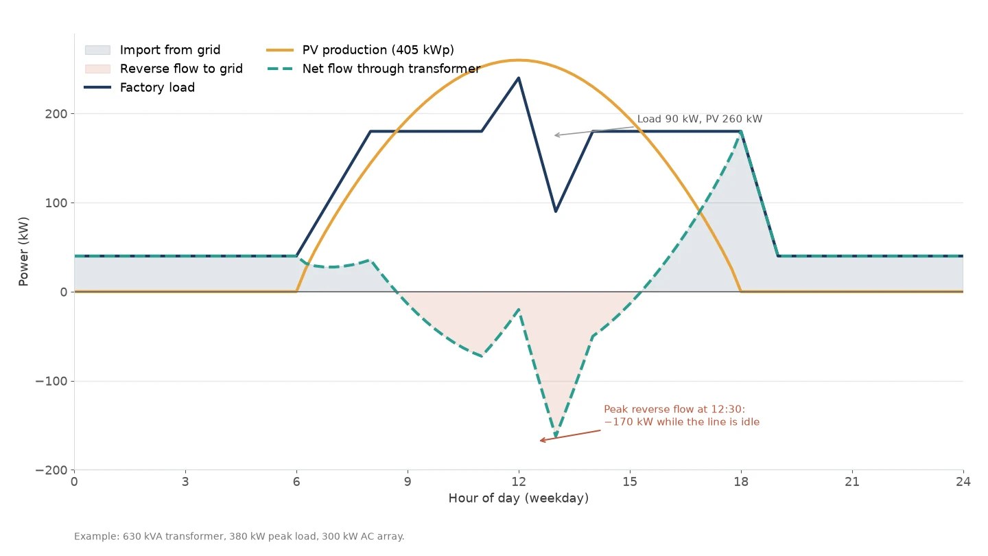
First, the transformer’s apparent power is not the sum of load and generation. When the load and the solar plant are on the same side of the transformer, they subtract. A 630 kVA transformer carrying a 380 kW load at 0.92 power factor is at 413 kVA, or 66% of rating. Add a 300 kW array producing at full output during that load, and the net flow through the transformer falls to about 98 kVA. The transformer is not stressed by the array; it is relieved by it.
Second, the plant introduces reverse flow. At noon on a Sunday, when the factory is closed and the roof is at full production, the transformer carries the array’s output backwards toward the grid. That flow is limited by the array’s AC rating divided by its power factor, and it must be checked against the transformer’s reverse capability, its protection settings and the utility’s rules on reverse power.
| Existing transformer | Load peak (at 0.92 PF) | Remaining capacity | Solar AC that fits before review |
|---|---|---|---|
| 400 kVA | 250 kW (272 kVA) | 128 kVA | About 120 kW |
| 630 kVA | 380 kW (413 kVA) | 217 kVA | About 205 kW |
| 1,000 kVA | 600 kW (652 kVA) | 348 kVA | About 330 kW |
| 1,600 kVA | 900 kW (978 kVA) | 622 kVA | About 590 kW |
The table is a screening test, not a design. A transformer can be loaded above 100% for short periods, its insulation ageing depends on temperature rather than on instantaneous loading, and many utilities accept a solar connection that pushes the reverse flow to the transformer’s rating. But a plant that requires a transformer upgrade moves from a four-month project to an eighteen-month one, and the upgrade cost lands on the developer.
Transformer and substation equipment is specified against the reverse flow case, not the load case, once a plant is added. The kVA rating, the tap changer, the protection relays and the cable sizing all follow from the same number.
String inverters own the 50 kW to 1 MW band
At this capacity band the choice is not really between string and central inverters. It is between string inverters and string inverters with a different architecture.
Central inverters — one large unit, 500 kW to several MW, feeding a single MPPT — make sense on flat, uniform, ground-mounted arrays where every module sees the same irradiance and the cable runs are long. A commercial roof is the opposite: multiple orientations, partial shading from parapets and rooftop equipment, modules spread across three or four roof sections, and no room for a 2-tonne inverter cabinet.
String inverters put an MPPT on every string pair, which is what multi-orientation roofs require. A 300 kW plant might use six 50 kW string inverters, each with two or three MPPTs, mounted near its own array. The loss from one shaded string stays inside its own MPPT instead of dragging down the whole plant.
| Configuration | MPPT count at 300 kW | Typical use | Weakness |
|---|---|---|---|
| Six 50 kW string inverters | 12–18 | Multi-orientation commercial roofs | More units to monitor and maintain |
| Three 100 kW string inverters | 6–9 | Large single-plane roofs | Coarser shade tolerance |
| One 300 kW central inverter | 1 | Flat ground-mounted arrays | Single point of failure; shade intolerant |
There is a real cost to the distributed approach: more devices, more AC combiner boxes, more communication points. The trade is justified whenever the roof has more than one orientation or any shading after 09:00, which describes most commercial roofs above 100 kW.
The practical sizing rule is to keep each inverter’s DC input between 1.1 and 1.4 times its AC rating, keep the string voltage inside the inverter’s window at the site’s lowest expected cell temperature, and keep the number of strings per MPPT even. The inverter selection itself is a second decision, made after the array and the transformer are fixed. The last rule prevents the mismatch loss that quietly eats 1 to 2% of yield on otherwise well-designed plants.
P90, not P50: size to the generation you can guarantee
Every yield estimate is a distribution, and the number that matters depends on who is asking.
P50 is the median: there is a 50% chance the plant produces more over its life and a 50% chance it produces less. P90 is the value exceeded in 90% of years, which is to say a 10% chance of falling short. The gap between them is typically 6 to 9% on a commercial plant, driven by year-to-year variation in irradiance and by uncertainty in the loss assumptions.
A developer selling a plant wants P50 or higher, because the buyer will compare it with other opportunities. A factory financing the plant against its own energy savings should size and model on P90, because the loan payment does not fall in a cloudy year.
The loss chain that separates array nameplate from delivered energy is well understood, and each step should be written into the calculation rather than applied as a single factor.
| Loss | Typical range | What drives it |
|---|---|---|
| Soiling and snow | 1–4% | Cleaning schedule, dust, tilt angle |
| Module temperature | 5–12% | Ambient temperature, mounting, module coefficient |
| Module mismatch | 1–2% | Binning quality, string design |
| DC cabling | 1–2% | Cable length and sizing |
| Inverter conversion | 1.5–3% | Load profile against efficiency curve |
| AC cabling and transformer | 1–2% | Distance to the point of connection |
| Availability | 0.5–1% | Maintenance, faults, grid outages |
A well-designed commercial plant lands at a performance ratio of 0.75 to 0.82. A proposal quoting 0.85 is either using optimistic inputs or has left a loss out, and the omission will surface as a shortfall in the first full year.
The same discipline applies to the degradation assumption. Modules lose about 0.5% of output per year under a typical warranty, and a 25-year average of 0.55% is defensible. A financial model that assumes no degradation over 20 years overstates lifetime yield by roughly 10%.
Power factor requirements shrink the AC side
The interconnection approval almost always specifies a power factor at the point of connection, commonly 0.95 lagging to 0.95 leading, and that requirement changes the equipment ratings you have to buy.
Inverters are rated in kVA, not kW. A 300 kW inverter operating at unity power factor delivers 300 kW. Asked to deliver the same 300 kW at 0.95 power factor, it must supply 316 kVA, which is above its rating if the unit is nameplate-rated at 300 kVA. The practical result is that a plant required to hold 0.95 at the point of connection loses about 5% of its usable active power unless the inverter is oversized or a separate reactive compensation unit is installed.
Two consequences follow. The transformer and AC cabling must be sized in kVA at the specified power factor, not in kW, or they will be undersized from the day of commissioning. And the inverter’s reactive capability has to be stated in the design, because many string inverters can absorb reactive power but at a reduced active output, and the reduced output is what the energy model must use.
Where the utility requires dynamic voltage support, a dedicated static compensator may be cheaper than oversizing every inverter on the roof. Where the requirement is a fixed power factor, setting the inverters to 0.95 is usually enough, provided the AC side was sized for it.
Worked example: a 300 kW factory rooftop, step by step

The example below is a real design sequence with the numbers left in, so the method can be checked and reused. The site is a factory in a high-irradiance region with a 630 kVA transformer, a 2,800 m² roof and an interconnection approval for 300 kW AC with zero export.
Step 1 — Fix the AC ceiling. The approval is 300 kW AC, zero export. This caps the inverter total at 300 kW and means any generation above site load is curtailed automatically.
Step 2 — Measure the load shape. The 15-minute data shows a weekday load of 180 kW from 08:00 to 18:00, a midday peak of 240 kW, a lunch dip to 90 kW, and 40 kW at night and on weekends. Annual consumption is 1.15 GWh.
Step 3 — Choose the DC/AC ratio. At 1.35, the array is 405 kWp against 300 kW of inverter. Modules of 580 W and 2.28 m² give 699 modules. The roof can hold them: 699 × 2.28 = 1,594 m² of module area, which fits inside 2,800 m² with room for walkways and parapet setbacks.
Step 4 — Check the transformer. Existing peak load is 380 kW at 0.92 power factor, or 413 kVA, which is 66% of the 630 kVA rating. The array’s output subtracts from the load during working hours. At 12:30 on a weekday, the line is idle at 90 kW while the array is at 260 kW, so the transformer carries 170 kW of reverse flow — 179 kVA at 0.95 power factor, or 28% of its rating. The transformer is never asked to carry more than about 66% in either direction. No upgrade is required.
Step 5 — Estimate production. Site irradiance is 1,650 kWh/m²/yr on the array plane. With a performance ratio of 0.80, annual output is:
405 kWp × 1,650 kWh/m²/yr × 0.80 = 534,600 kWh
That is the P50 value. Applying a P90 factor of 0.94 gives 502,500 kWh, which is the number to use for the financing case.
Step 6 — Compute self-consumption. Matching 15-minute generation against 15-minute load, with the zero-export controller clipping output to load, gives a self-consumption rate of 58%. Of the 535 MWh generated, 310 MWh is consumed on site and 225 MWh is curtailed — mostly at weekends and during the lunch dip, when the roof is producing and the factory is not.
Step 7 — Value the energy. At a retail tariff of USD 0.18/kWh and a feed-in tariff of USD 0.06/kWh — and with export prohibited, so the surplus is worth nothing — annual savings are:
310,000 kWh × USD 0.18 = USD 55,800 per year
The curtailed 225 MWh represents USD 40,500 of annual value that the zero-export rule simply removes. That number is the business case for storage, and it is exactly why the next section exists.
Step 8 — Check the AC side at the required power factor. The utility requires 0.95 at the point of connection. The 300 kW inverter must supply 316 kVA, and the AC cabling and the connection point are sized for that. Because the transformer already has 217 kVA of headroom, the reactive requirement does not force an equipment change.
The complete configuration: 405 kWp of modules, 300 kW of string inverters with 12 MPPTs, zero-export control, 630 kVA transformer retained, and a measured self-consumption rate of 58%.
Interconnection checklist: protection, metering, communication
Interconnection delays are rarely technical. They are almost always documentation, and every item on the list below has to be produced by someone before the utility will energize the plant.
| Item | Produced by | Typical lead time |
|---|---|---|
| Single-line diagram of the plant and connection point | EPC or designer | 1–2 weeks |
| Protection coordination study and relay settings | Protection engineer | 3–6 weeks |
| Inverter test certificates and grid-code compliance | Equipment supplier | 1–3 weeks |
| Metering arrangement, CT/PT ratios, meter type | Utility and installer | 2–4 weeks |
| Load flow and short-circuit study | Consultant | 4–8 weeks |
| Commissioning and witness test procedure | EPC and utility | 2–4 weeks |
| As-built documentation and protection test records | EPC | At handover |
The two items that most often extend a schedule are the protection study and the metering arrangement. The protection study depends on the utility’s fault level data, which the utility may take weeks to release. The metering arrangement depends on whether the utility accepts a bidirectional meter with the required accuracy class, and on whether it will accept the inverter’s own export limitation or insists on a contactor-based interlock.
Bring both into the conversation at the feasibility stage, not at the commissioning stage. Roof condition and access will shape the construction sequence; the interconnection package shapes whether the plant is allowed to run at all.
When self-consumption falls below 60%, add storage
A self-consumption rate below 60% is the point where a grid-tied plant starts leaving money on the roof, and storage becomes the cheaper way to recover it.
The arithmetic is the same as in the worked example. Every kilowatt-hour generated and not consumed on site is worth the feed-in tariff — and under a zero-export approval, worth nothing. A battery moves that energy from midday to the evening, where it displaces retail-priced consumption, and the value of the move is the retail tariff minus the round-trip loss.
Sizing the battery is a matter of matching daily surplus, not annual surplus. In the example, the 225 MWh of annual curtailment spreads unevenly: weekends produce large surpluses, weekdays produce small ones. A 300 kWh battery charged and discharged once per day absorbs about 100 MWh a year at an 85% round-trip efficiency, recovering roughly 44% of the curtailed energy for a fraction of the cost of a second array.
Two rules keep the battery from being oversized. Size it to the daily surplus on a typical weekday, not the worst weekend. And size it to the evening load it will serve, because a battery that can store more than the evening load can use is a battery that sits full.
A solar plus battery configuration is the natural next step when the export limit is zero and the daytime load is smaller than the roof. The kW and kWh of that battery are decided by the evening load and the daily surplus respectively, not by the array size.
The capacity is the smallest of four numbers
A grid-tied solar plant at 50 kW to 1 MW is sized by whichever of these four is smallest:
1. The AC capacity the utility will approve, including its export rule.
2. The transformer’s remaining capacity in kVA, checked in both directions.
3. The roof or land area after setbacks, shading and walkways.
4. The load that can absorb the output, measured in 15-minute intervals.
The inverter ratio and the module count come after all four. They are the last decisions in the sequence, not the first, and a design that begins with the module count will eventually meet one of the four ceilings and lose the value it was supposed to create.
Module selection matters, but it is worth less than getting the four ceilings right. A 300 kW plant on 20% less efficient modules loses 3% of yield; a 300 kW plant that ignored a 150 kW export limit loses 40% of its business case.
FAQ
– Q: How many panels do I need for a 500 kW solar plant? A: For a 500 kW AC plant at a DC/AC ratio of 1.3, you need 650 kWp of modules. At 580 W per module that is 1,120 modules, covering roughly 2,550 m² including walkways and setbacks. The module count is the output of the sizing process, not the input.
– Q: What DC/AC ratio should I use? A: Between 1.15 and 1.35 for most commercial roofs, with 1.35 acceptable where the inverter is mounted in a cool location and the utility does not define capacity by inverter rating. Above 1.5 the clipping loss grows faster than the module savings.
– Q: Can I export surplus power to the grid? A: Only if the interconnection approval permits it. Many networks now issue zero-export approvals for new commercial plants, which makes storage the only way to use surplus midday production. Confirm the export rule before sizing the array.
– Q: How long does grid interconnection approval take? A: Typically three to nine months for a commercial plant in this range, of which the technical review is usually the shorter part. The protection study and the metering agreement are the items that extend it, and both depend on documents the utility releases on its own schedule.
– Q: What is the smallest load that justifies a 1 MW plant? A: A site needs roughly 700 to 900 kW of daytime load to absorb a 1 MW plant without export, or an export approval. Below that, the plant either spills most of its output or needs a battery sized to the midday surplus. We size these projects from the load curve, and a 15-minute data set is the best place to start.
YURI POWER Engineering Team · November 19, 2026